Acceleration with HLS - Load, Compute, Store

In my daily work on FPGAs for the CMS Level 1 Trigger we usually are not limited by I/O into the devices. We work with boards, like the Serenity and APx, which can support 4-5 Tb/s input on around 100 optical fibres with very low latency - 100 ns or so for a hop from one board to the next. This is very convenient for designing algorithms, since often all (or at least many) of the inputs can be accessed in parallel through registers. We often quote throughput and latency numbers for algorithms or IPs inside the FPGA without discussing the interface, since it’s so fast. Some of my projects relate to hardware acceleration, however, and here I usually need to think a lot more about data movement from the outside world (the host) to the device, and back.
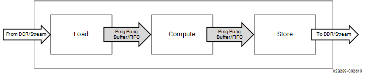
In that context I recently refactored some code in the conifer library for BDTs to properly make use of the load, compute, store pattern advised by AMD/Xilinx. Using this design pattern, one should partition the code into distinct load, compute, and store functions, using streams to pass data between them and applying dataflow at the top level. In conifer, the compute is a BDT inference, while the load and store read and write data from an AXI master interface. I’ve been targeting an Alveo U200 device that I use for development and testing, so this interface is connected to the card DDR memory and accessed via DMA with the host. Importantly for the conifer accelerator implementation, the HLS kernel takes the number of samples N as a runtime variable and loops over the samples internally. I wanted to make sure that the kernel properly pipelines the load, compute, and store tasks, to achieve a high throughput. And it turns out that the code in the library so far doesn’t achieve the best performance that it could! This development targets the xilinxhls backend of conifer, which implements the specific BDT model into the generated IP, along with the wrapper with AXI interfaces for acceleration. This differs a bit from the FPU backend which, while also implemented in HLS, is a bit more complicated due to the reusability of the IP for different BDT models.
Here’s the diagram from AMD’s documentation that I was aiming for (credit AMD UG1393):
I started from conifer’s sklearn_to_hls.py example, modified to target the Alveo U200:
from sklearn.datasets import make_hastie_10_2
from sklearn.ensemble import GradientBoostingClassifier
import conifer
import datetime
import numpy as np

import sys
import logging
logging.basicConfig(stream=sys.stdout, level=logging.WARNING)
logger = logging.getLogger('conifer')
logger.setLevel(logging.DEBUG)

# Make a random dataset from sklearn 'hastie'
X, y = make_hastie_10_2(random_state=0)
X_train, X_test = X[:2000], X[2000:]
y_train, y_test = y[:2000], y[2000:]

# Train a BDT
clf = GradientBoostingClassifier(n_estimators=20, learning_rate=1.0,
                                 max_depth=3, random_state=0).fit(X_train, y_train)

# Create a conifer config
cfg = conifer.backends.xilinxhls.auto_config()
# Set the output directory to something unique
cfg['OutputDir'] = 'prj_sklearn_u200'
cfg['AcceleratorConfig'] = {'InterfaceType' : 'float',
                            'Board' : 'xilinx_u200_gen3x16_xdma_2_202110_1'}

# Create and compile the model
model = conifer.converters.convert_from_sklearn(clf, cfg)
model.compile()

# Run HLS C Simulation and get the output
y_hls = model.decision_function(X)
y_skl = clf.decision_function(X)

# Synthesize the model
model.build(bitfile=True)
I built two bitfiles for the model: using the v1.8 release of conifer, and a development branch pyxrt where I refactored for the load, compute, store pattern. The BDT model is the same, only the top-level wrapper files are different. The full code is below, but in brief, the main differences between the two implementations are:
- use of streams (or no streams) to pass data between the load/compute/store functions
- and use of
#pragma HLS dataflowat the top level
- and use of
- different loops over
N:- v1.8 release:
for(n in N) load1(); compute1(); store1() pyxrtbranch:load(N); compute(N); store(N);- each function loops over N
- v1.8 release:
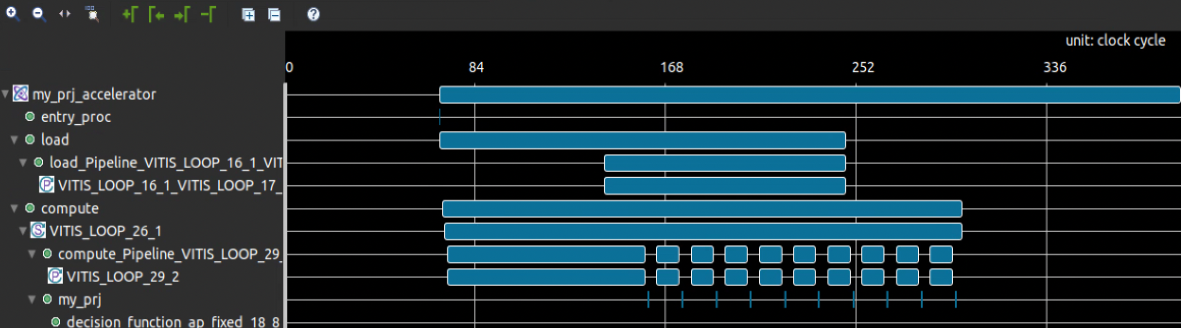
Cosimulation
In the cosimulation view we can see that the tasks are properly scheduled with overlapping execution only in the load/compute/store implementation (note the much longer execution time in case 1).
1 v1.8 release - mixed loading, computing, storing
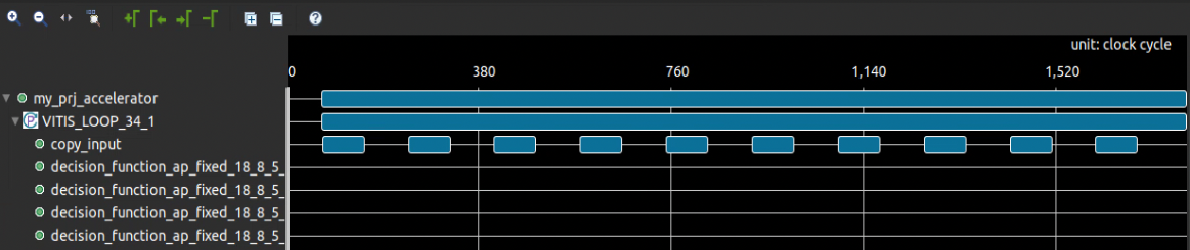
2 pyxrt branch - proper load / compute / store
Hardware performance
The two designs were built for Alveo U200 and tested on hardware. In both cases I used a new PyXrtAlveoDriver that I’m developing on the pyxrt branch of conifer - so that any differences in performance are only due to the kernel. The dataset has 10 features (variables) per example, as float32 type. I ran inference in a loop with different N samples, so that the trend can be seen, using the Python %%timeit magic which repeats the test multiple times. Here’s the timing test code (executed in ipython for the %timeit magic):
log10ns = np.linspace(0,4,30)           # log10(N) sample size with equal spacing for a log10 axis
N = np.floor(10**log10ns).astype('int') # N samples per trial
t = np.zeros(log10ns.shape)             # container for the timing results

# load the xclbin onto Alveo card
device = conifer.backends.xilinxhls.runtime.PyXrtAlveoDriver('./my_prj.xclbin', 0, 'my_prj_accelerator', 10, 1, 10000)

# run the timing tests
for i, n in tqdm(enumerate(N)):
  device._init_buffers(n) # resize the buffers to the sample size to time only the inference execution for N samples
  Xn = X[:n]              # slice n samples
  result = %timeit -o device.decision_function(Xn) # time the inference on device, %timeit runs multiple trials
  t[i] = result.average                            # capture the average result from the trials
Here are the results from running the same test twice, targeting the xclbin built with the v1.8 release and the pyxrt branch with properly implemented load, compute, store pattern.
The y-axis on the top panel is total inference time, so lower values are better. In the bottom panel you see the ratio of time from the release over the time from the branch implementation, so higher values are better.
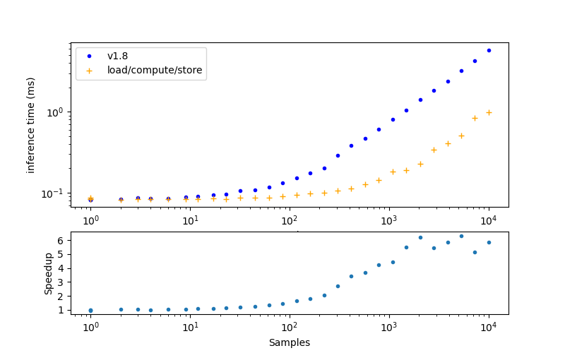
You can see that the properly implemented pattern is faster than the release across all sample sizes, besides N=1, where the performance is the same. The speedup is most visible with larger sample sizes as we get further away from the 80 μs floor that seems to be the fastest time we can do anything on the device.
With 10,000 examples on the pyxrt branch, the total inference time is 0.99 ms, giving 10,100,000 examples per s or 99 ns per example, and a speedup of 5.8x over the v1.8 implementation!
These improvements will be made available in the conifer v1.9 release! The next step is to check if the same improvement can be made to the FPU backend.
Top level code
1 v1.8 release - mixed loading, computing, storing
#include "BDT.h"
#include "parameters.h"
#include "my_prj.h"

void my_prj(input_arr_t x, score_arr_t score){
  #pragma HLS array_partition variable=x
  #pragma HLS array_partition variable=score
  #pragma HLS pipeline
  #pragma HLS unroll
  bdt.decision_function(x, score);
}

void copy_input(int n, accelerator_input_t* x_in, input_arr_t x_int){
  for(int i = 0; i < n_features; i++){
    x_int[i] = x_in[n_features*n + i];
  }
}

void copy_output(int n, score_arr_t score_int, accelerator_output_t* score_out){
  for(int i = 0; i < BDT::fn_classes(n_classes); i++){
    score_out[BDT::fn_classes(n_classes)*n + i] = score_int[i];
  }
}

void my_prj_accelerator(int N, int& n_f, int& n_c, accelerator_input_t* x, accelerator_output_t* score){
  #pragma HLS interface mode=m_axi port=x offset=slave bundle=gmem0
  #pragma HLS interface mode=m_axi port=score offset=slave bundle=gmem0
  #pragma HLS interface mode=s_axilite port=N
  #pragma HLS interface mode=s_axilite port=n_f
  #pragma HLS interface mode=s_axilite port=n_c
  n_f = n_features;
  n_c = BDT::fn_classes(n_classes);
  for(int n = 0; n < N; n++){
    #pragma HLS pipeline
    input_arr_t x_int;
    score_arr_t score_int;
    copy_input(n, x, x_int);
    bdt.decision_function(x_int, score_int);
    copy_output(n, score_int, score);
  }
}
2 pyxrt branch - proper load / compute / store
#include "BDT.h"
#include "parameters.h"
#include "my_prj.h"
#include "hls_stream.h"

void my_prj(input_arr_t x, score_arr_t score){
  #pragma HLS array_partition variable=x
  #pragma HLS array_partition variable=score
  #pragma HLS pipeline
  #pragma HLS unroll
  bdt.decision_function(x, score);
}

void load(int N, accelerator_input_t* x, hls::stream<input_t>& x_stream){
  for(int n = 0; n < N; n++){
    for(int i = 0; i < n_features; i++){
      #pragma HLS pipeline
      input_t xi = x[n * n_features + i];
      x_stream.write(xi);
    }
  }
}

void compute(int N, hls::stream<input_t>& x_stream, hls::stream<score_t>& score_stream){
  for(int n = 0; n < N; n++){
    input_arr_t x_int;
    score_arr_t score_int;
    for(int i = 0; i < n_features; i++){
      #pragma HLS pipeline
      x_int[i] = x_stream.read();
    }
    my_prj(x_int, score_int);
    for(int i = 0; i < BDT::fn_classes(n_classes); i++){
      #pragma HLS pipeline
      score_stream.write(score_int[i]);
    }
  }
}

void store(int N, hls::stream<score_t>& score_stream, accelerator_output_t* score){
  for(int n = 0; n < N; n++){
    for(int i = 0; i < BDT::fn_classes(n_classes); i++){
      #pragma HLS pipeline
      score_t scorei = score_stream.read();
      score[n * BDT::fn_classes(n_classes) + i] = scorei;
    }
  }
}

void my_prj_accelerator(int N, int& n_f, int& n_c, accelerator_input_t* x, accelerator_output_t* score){
  #pragma HLS interface mode=m_axi port=x offset=slave bundle=gmem0
  #pragma HLS interface mode=m_axi port=score offset=slave bundle=gmem0
  #pragma HLS interface mode=s_axilite port=N
  #pragma HLS interface mode=s_axilite port=n_f
  #pragma HLS interface mode=s_axilite port=n_c
  #pragma HLS dataflow
  n_f = n_features;
  n_c = BDT::fn_classes(n_classes);

  hls::stream<input_t> x_stream("x_stream");
  hls::stream<score_t> score_stream("score_stream");
  #pragma HLS STREAM variable=x_stream depth=1024
  #pragma HLS STREAM variable=score_stream depth=1024

  load(N, x, x_stream);
  compute(N, x_stream, score_stream);
  store(N, score_stream, score);
}